Customer lifetime value

This is for:

Developer

In this article

What’s in this article?
Intro
Input data
Model
Predictions
Example use cases
Getting started

In this article, we will look at the Customer Lifetime Value (CLV) model and how you can use it to predict visitor behavior.

What’s in this article?

We will provide an overview of how this model is built, its data requirements, and the predictions it can make. We will also provide details of use cases showing how this model can be integrated into your personalization efforts.

In particular, we will cover:

What our CLV model predicts
What it uses to make that prediction
Some potential use cases
How you can reach out to Qubit should you be interested in using the model to power your experiences

Intro

The CLV model is a custom-built machine learning model that predicts the future spend for each customer–a person that has converted at least once–over a specified time horizon. Also, it estimates the churn probability, future purchase frequency, and future Average Order Value (AOV) for each customer.

The features used to train this model are constructed from a visitor’s previous transaction history and can be provided from a number of sources, including QProtocol or your own CRM/CDP system.

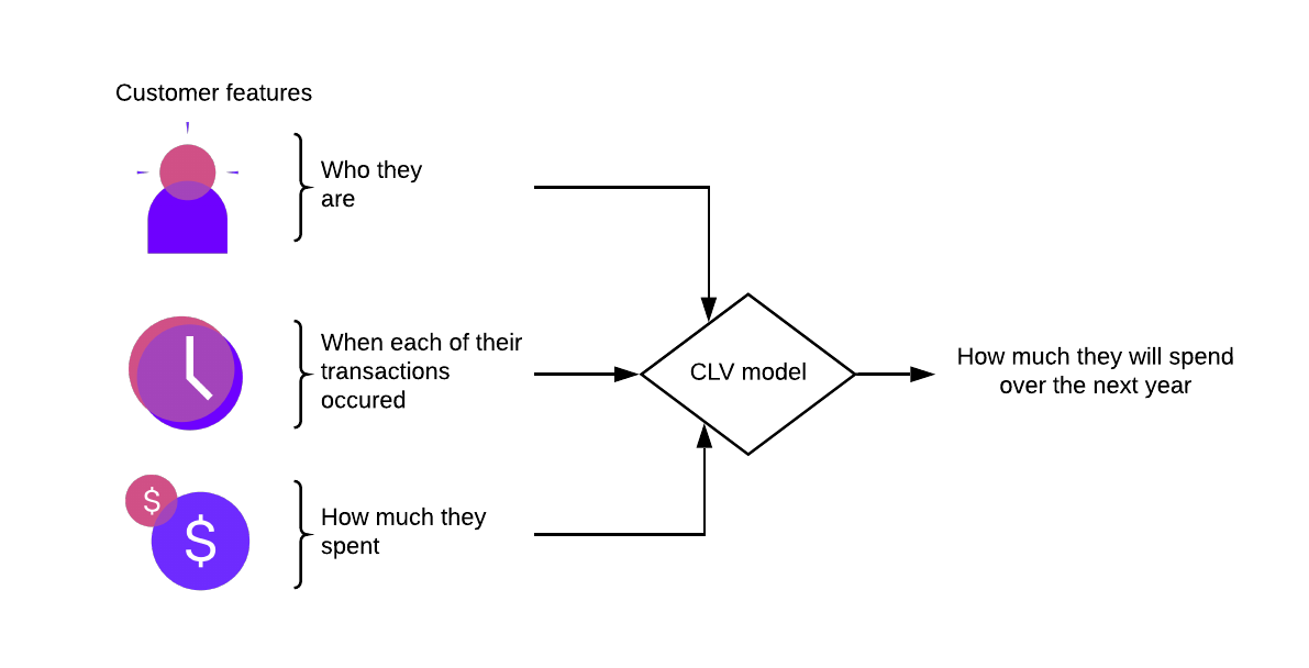
The following diagram provides a high-level overview of how this model functions:

Input data

The model needs three data points for each historic transaction:

A unique customer identifier - User email or context Id
The time of the transaction
The transaction value or amount spent

All three of these are required for the model to function and can be provided from a number of sources, including QProtocol (QP), GA360, or your own CRM or CDP system.

The following table summarizes the data requirements for each data point:

Customer identifier	Data source	Vertical	QP Event(s)	Timestamp field	Order value field
context_id	QP	ec	event_ecBasketTransactionSummary	meta_serverTs	basket_total_baseValue
context_id	QP	tr	event_trPackageTransactionSummary	meta_serverTs	package_total_baseValue
context_id	QP	eg	event_egGamePlay	meta_serverTs	playValue_baseValue
user_email	QP	ec	event_ecBasketTransactionSummary, event_ecView,event_ecUser	meta_serverTs	basket_total_baseValue
user_email	QP	tr	event_trPackageTransactionSummary, event_trView,event_trUser	meta_serverTs	package_total_baseValue
clientId	GA360	n/a	n/a	visitStartTime	totals.totalTransactionRevenue
varies	CRM/CDP	n/a	n/a	varies	varies

Customer identifier

Data source

Vertical

QP Event(s)

Timestamp field

Order value field

context_id

event_ecBasketTransactionSummary

meta_serverTs

basket_total_baseValue

context_id

event_trPackageTransactionSummary

meta_serverTs

package_total_baseValue

context_id

event_egGamePlay

meta_serverTs

playValue_baseValue

user_email

event_ecBasketTransactionSummary, event_ecView,event_ecUser

meta_serverTs

basket_total_baseValue

user_email

event_trPackageTransactionSummary, event_trView,event_trUser

meta_serverTs

package_total_baseValue

clientId

GA360

n/a

visitStartTime

totals.totalTransactionRevenue

varies

CRM/CDP

n/a

varies

If one or more of the feature fields are missing or invalid, the model will often continue to operate, but with less input information, which can lead to lower accuracy.

Note

We rely on historical customer behavior to train the model and make accurate predictions. Typically you should have training data that goes back as far into the past as you would want to predict into the future. For example, if you want to predict one year into the future, you need one year’s worth of past data.

Model

The CLV model uses a Bayesian hierarchical framework to infer three parameters:

Churn probability
Effective Frequency
Average (mean) transaction value

Mean transaction value predicts how much each customer will spend, on average, in each future transaction. Churn probability and effective frequency are strongly related and can be illustrated by the following example.

Note

A customer converted three times, starting one year ago and ending after six months. Their historical order frequency is three per year. However, because the customer stopped buying six months ago, it’s more likely the actual (or effective) frequency is six per year; to this, we would also posit that the customer has a high churn probability– the customer has probably churned.

Because churn is not observed in non-contractual settings, the model must be realistic enough to infer this latent variable by teasing apart churn and effective frequency.

Bayesian hierarchical modeling is a method of statistical modeling composed of multiple levels (hierarchies) that uses Bayes’s rule to estimate probability distributions using a combination of prior knowledge and observed data. Our CLV model has been crafted by our expert team of data scientists to ensure the best possible performance.

Our models produce high predictive accuracy relative to the domain. We measure predictive performance using a metric known as mean absolute error. Our models typically achieve a mean absolute error around 50x smaller than a benchmark model that takes the amount spent by customers in the past and extrapolates this into the future.

For example, the mean absolute error of the model could be around USD 92, with an average observed yearly transaction value of about USD 36. That error is significant compared with the actual average, but it’s still much better than simple extrapolation. Moreover, the error is mainly due to one-time purchasers that never buy again; for customers with even moderate loyalty, the model is far more accurate.

Predictions

Each customer’s CLV is calculated daily or weekly by a batch job. This job outputs timestamped estimates of CLV and its component parameters into a table in the client’s BigQuery project, for example,clientName__v2.clv_output_user_email.

In addition to CLV, several other (derived) quantities are calculated:

Churn probability over a month - this uses the churn probability parameter to forecast churn over time
Expected time until churn - the expected time it will take until the customer churns
Expected number of purchases - this is a direct input to CLV
Inter purchase time - the average time between purchases (inverse of effective frequency parameter)
Spent per purchase - this equals the average transaction value parameter and is a direct input to CLV

For each of these, alongside the prediction, two percentile columns are provided to indicate the degree of uncertainty in the predictions. Finally, we show the data that were used to train the model as well.

The following table provides a detailed overview of the output in the client project. This output can be actioned by using a Derived Dataset (DD).

Column name	Description	Type	Example
customer_id	user_email	STRING	abc@gmail.com
total_order_value	The total order value (input data)	FLOAT	56.0
n_purchases	The number of purchases (input data)	INT	1
recency	Time of last purchase (somewhere between zero and 'horizon'; input data)	FLOAT	0.0
horizon	Time since first purchase (in months; input data)	FLOAT	33.6594077660032
churn_prob_month_pred	The median (prediction) for monthly churn probability	FLOAT	0.950173113021867
churn_prob_month_5th_perc	The 5th percentile (low-end) for monthly churn probability	FLOAT	0.600931490503537
churn_prob_month_95th_perc	The 95th percentile (high-end) for monthly churn probability	FLOAT	0.999331135251575
time_until_churn_pred	The median (prediction) for time until churn	FLOAT	13.695012237352
time_until_churn_5th_perc	The 5th percentile (low-end) for time until churn	FLOAT	0.254433688275367
time_until_churn_95th_perc	The 95th percentile (high-end) for time until churn	FLOAT	2828.65668852401
n_purchases_pred	The median (prediction) for number of purchases over one year	FLOAT	0.169668618831138
n_purchases_5th_perc	The 5th percentile (low-end) for number of purchases over one year	FLOAT	0.0068908852383051
n_purchases_95th_perc	The 95th percentile (high-end) for number of purchases over one year	FLOAT	1.17028945948419
inter_purchase_time_pred	The median (prediction) for inter purchase time	FLOAT	18.2889708302299
inter_purchase_time_5th_perc	The 5th percentile (low-end) for inter purchase time	FLOAT	2.40946077083366
inter_purchase_time_95th_perc	The 95th percentile (high-end) for inter purchase time	FLOAT	329.870692032285
spent_per_purchase_pred	The median (prediction) for spent per purchase	FLOAT	58.2994385267867
spent_per_purchase_5th_perc	The 5th percentile (low-end) for spent per purchase	FLOAT	36.0385163299792
spent_per_purchase_95th_perc	The 95th percentile (high-end) for spent per purchase	FLOAT	96.2416328688191
clv_pred	The median (prediction) for clv	FLOAT	9.86300874365342
clv_5th_perc	The 5th percentile (low-end) for clv	FLOAT	0.278750968839795
clv_95th_perc	The 95th percentile (high-end) for clv	FLOAT	71.1121355784755
prediction_date	The date when the predictions were calculated (same for all in a given batch)	STRING	2020-01-13

Column name

Description

Type

Example

customer_id

user_email

STRING

abc@gmail.com

total_order_value

The total order value (input data)

FLOAT

56.0

n_purchases

The number of purchases (input data)

INT

recency

Time of last purchase (somewhere between zero and 'horizon'; input data)

FLOAT

0.0

horizon

Time since first purchase (in months; input data)

FLOAT

33.6594077660032

churn_prob_month_pred

The median (prediction) for monthly churn probability

FLOAT

0.950173113021867

churn_prob_month_5th_perc

The 5th percentile (low-end) for monthly churn probability

FLOAT

0.600931490503537

churn_prob_month_95th_perc

The 95th percentile (high-end) for monthly churn probability

FLOAT

0.999331135251575

time_until_churn_pred

The median (prediction) for time until churn

FLOAT

13.695012237352

time_until_churn_5th_perc

The 5th percentile (low-end) for time until churn

FLOAT

0.254433688275367

time_until_churn_95th_perc

The 95th percentile (high-end) for time until churn

FLOAT

2828.65668852401

n_purchases_pred

The median (prediction) for number of purchases over one year

FLOAT

0.169668618831138

n_purchases_5th_perc

The 5th percentile (low-end) for number of purchases over one year

FLOAT

0.0068908852383051

n_purchases_95th_perc

The 95th percentile (high-end) for number of purchases over one year

FLOAT

1.17028945948419

inter_purchase_time_pred

The median (prediction) for inter purchase time

FLOAT

18.2889708302299

inter_purchase_time_5th_perc

The 5th percentile (low-end) for inter purchase time

FLOAT

2.40946077083366

inter_purchase_time_95th_perc

The 95th percentile (high-end) for inter purchase time

FLOAT

329.870692032285

spent_per_purchase_pred

The median (prediction) for spent per purchase

FLOAT

58.2994385267867

spent_per_purchase_5th_perc

The 5th percentile (low-end) for spent per purchase

FLOAT

36.0385163299792

spent_per_purchase_95th_perc

The 95th percentile (high-end) for spent per purchase

FLOAT

96.2416328688191

clv_pred

The median (prediction) for clv

FLOAT

9.86300874365342

clv_5th_perc

The 5th percentile (low-end) for clv

FLOAT

0.278750968839795

clv_95th_perc

The 95th percentile (high-end) for clv

FLOAT

71.1121355784755

prediction_date

The date when the predictions were calculated (same for all in a given batch)

STRING

2020-01-13

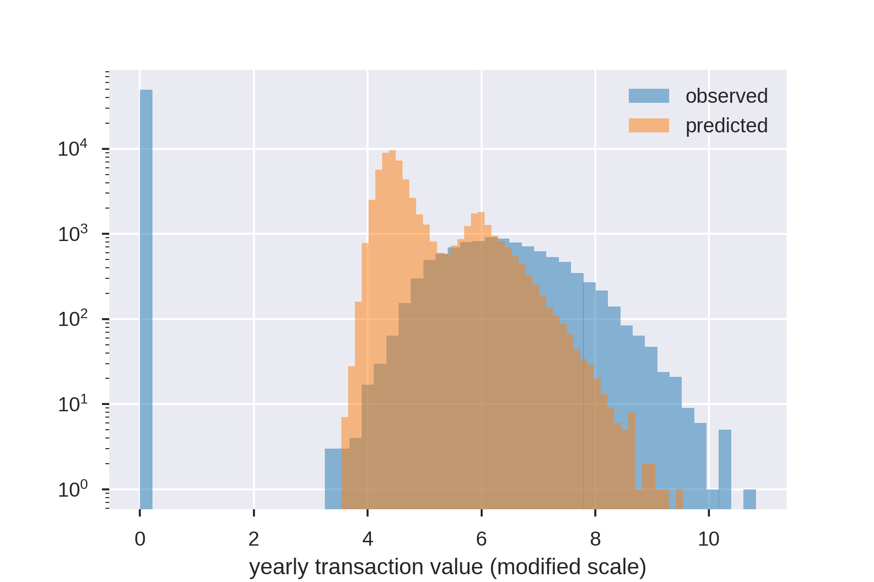
In the following image, the predictions, clv_pred and realizations–what has actually been observed, are plotted for a client with a period of 12 months and user_email as primary key. The model is able to capture the fact that there are two peaks in the distribution, corresponding to one-time purchasers and the average, loyal customer.

Example use cases

There are many use cases for CLV, including segmentation, investment decisions, and optimization.

Segmentation

Customers can be segmented based off of CLV, for example, into low, medium, and high-value customers. This could inform a loyalty program, and it could even be used to promote loyalty program signup for high-value customers.

Moreover, CLV segments could be an alternative to commonly used Recency, Frequency, and Monetary (RFM) based segments because it is a compression of RFM into a single, predictive number, hence simpler to segment on. For example, you could provide Unique Selling Proposition messaging or trending products to customers with a low CLV.

Investment decisions

Because companies have limited resources, it is important to know how to allocate marketing spend. CLV can help determine which advertising channels to invest in and how much to spend. In the context of CRM marketing, it could aid in deciding who to send discount vouchers to, by, for example, targeting valuable high CLV customers or basing the voucher amount on CLV. Clearly, you would not want to give customers a discount that is bigger than their future spend. It is even possible to improve customer service by prioritizing high CLV customers.

Aside from CLV, segmentation can be applied to any of the three parameters, particularly churn probability. Once you know which customers are at high risk of churning, you can target them with discounts or other offers. It can also be useful to combine these use cases with CLV-based ones. For example, if you segment on both churn probability and CLV, you will automatically find the at-risk customers that are valuable enough for marketing to invest in. This way, one model gives four (smart) attributes to create audiences.

Optimization

As total CLV is a measure of long term revenue, it is closely related to long term profits–a strategic objective, and most definitely a quantity businesses would want to optimize. Therefore, in the future, it could be used as a goal for the traditional optimization offered by A/B testing, the automatic optimization offered by Multi-Armed Bandits, or more sophisticated methods. However, these are not use cases we currently support. It can also be used in reporting for businesses that wish to track movements.

More broadly, use cases can be joined. Suppose customers are segmented based on their CLV. One could then try to improve loyalty by trying to move customers from the low CLV segment into the medium CLV segment, etc. This makes the model useful for both segmentation and optimization.

Getting started

To start using this model in Qubit experiences, contact your Customer Success Manager and ask for the early access signup form. Submit this form and enter CLV as the project name you’re interested in.